Example 7: JARUS model vs the iGRC values

In this example we compare the iGRC table in Annex F with the actual output of the JARUS model. This is done by plotting the critical area for a variety of wingspan and population densities. This is similar to the iGRC figures that can be computed with the Figures class, which do the same thing, but for the simplified model.

First, we need to set the impact angle. This is not used in the simplified model, where the impact angle has been simplified away. However, for the JARUS model we need to set this, since the critical area depends on it. Here we choose default value from AnnexFParms (35 degrees) since this angle has a specific meaning in Annex F. But any angle will do, but obviously produce a slightly different plot. Also note that the impact speed may vary with the impact angle.

impact_angle = AnnexFParms.scenario_angles[1]

We instantiate the CA model class.

CA = CriticalAreaModels()

We set the sampling density for the two axes.

pop_density_samples = 400
wingspan_samples = 200

We set the arrays for the sampling on the two axes. Note that the wingspan axis is linear, while the population density axis is logarithmic.

wingspan = np.linspace(0, 21, wingspan_samples)
pop_density = np.logspace(-3 + np.log10(5), 6, pop_density_samples)

We instantiate the Annex F parmeters class AnnexFParms.

Initialize the background matrix with zeros.

GRC_matrix = np.zeros((pop_density_samples, wingspan_samples))

We run a for loop over the range of the wingspan.

for j in range(len(wingspan)):

Now, for every value of the wingspan, we want to use the aircraft values associated with the wingspan, i.e., the appropriate column in the iGRC table.

    if wingspan[j] <= AFP.CA_parms[0].wingspan:
        column = 0
    elif wingspan[j] <= AFP.CA_parms[1].wingspan:
        column = 1
    elif wingspan[j] <= AFP.CA_parms[2].wingspan:
        column = 2
    elif wingspan[j] <= AFP.CA_parms[3].wingspan:
        column = 3
    else:
        column = 4

Since we previously set the impact angle to 35 degrees, we will use the cruise speed as impact speed.

    impact_speed = AFP.CA_parms[column].cruise_speed

However, if we had chosen another angle, we would consider using another speed. Specificallty, in Annex F it is assumed that for an impact at 10 degrees, the speed is reduced equivalent to multiplying with a factor 0.65. This glide speed value can also be obtained from the AFP class as AFP.CA_parms[column].glide_speed.

We set the wingspan according to the maximum value from each class.

    AFP.CA_parms[column].aircraft.width = wingspan[j]

We then compute the size of the critical area using the standard values from Annex F. Since there is no deflagration, the overlap is set to zero.

    M = CA.critical_area(AFP.CA_parms[column].aircraft, impact_speed, impact_angle)[0]

Finally, we populate the background matrix for the plot, that is the iGRC values associated with the combination of population density and critical area.

    for i in range(len(pop_density)):
        GRC_matrix[i, j] = AnnexFParms.iGRC(pop_density[i], M)[0]

Note that the [0] at the end selects the raw iGRC value, while a [1] would select the rounded up iGRC value.

This is followed by numerous lines for creating the plot. This includes showing the matrix along with contours, setting the tick locations and labels, and white lines and text for overlaying the iGRC. The result is as follows.

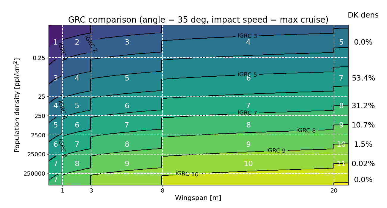
The iso-parametric curves in black show where the iGRC value has exactly integer values in the background plot. So for instance the curve for iGRC 9 is the boundary between values below 9 and above 9.

The percent of area in Denmark which corresponds to the different population density bands is also shown. These values are based on locations of addresses and a grid size of 1 km by 1 km. This information does not come from CasEx, and is just hardcoded into this example.