Example 6: Ballistic descent
This example shows how to compute a series of values for a ballistic descent. The same approach is used in Annex F for computing the ballistic values found in Appendix A.
The class BallisticDescent2ndOrderDragApproximation
is based on [2], which also
describes the detail on how the ballistic descent model works.
We first instantiate the class.
BDM = BallisticDescent2ndOrderDragApproximation()
We set the standard aircraft parameters
aircraft_type = enums.AircraftType.FIXED_WING
width = 2.8
mass = 90
and instantiate the aircraft class.
aircraft = AircraftSpecs(aircraft_type, width, mass)
We need to set the drag coefficient and the frontal area, since they are used in the computation of the ballistic descent. The drag coefficient is typically in the range from 0.7 to around 1 for an aircraft which is not descending “nicely”, i.e., in its usually direction of travel. Here we assume a normal helicopter-like rotorcraft, which may be tumbling during descent. We guestimate the coeffient to be 0.8. A lower coefficient would give a higher impact speed, and thus be more conservative. But 0.8 is not unreasonable for a tumbling rotorcraft. See for instance the wiki page on drag coefficient for more detail on drag for various shapes.
The frontal area is the area covered by the aircraft in the direction of travel during descent. Here we guess that it will be 60 cm by 60 cm, which is reasonable for a 90 kg aircraft.
aircraft.set_ballistic_drag_coefficient(0.8)
aircraft.set_ballistic_frontal_area(0.6 * 0.6)
The ballistic descent class must “be aware” of the aircraft.
BDM.set_aircraft(aircraft)
We also set the initial values for the descent, namely the altitude above the ground and the velocity of the aircraft at the beginning of the descent.
altitude = 100
initial_velocity_x = 28
initial_velocity_y = 0
We can now compute the ballistic descent.
p = BDM.compute_ballistic_distance(altitude, initial_velocity_x, initial_velocity_y)
- Note that p is a list with various values about the descent. Note also that
BDM has additional values (attributes) available, relating to the intermediate
computations as decribed in [2]. All available values are printed to the screen here.
print("Distance:     {:1.1f} m    ".format(p[0]))
print("Impact speed: {:1.1f} m/s".format(p[1]))
print("Angle:        {:1.1f} degs".format(p[2] * 180 / np.pi))
print("Time :        {:1.2f} s".format(p[3]))
print("Distances:    {:1.3f}  {:1.3f}  {:1.3f}".format(BDM.distance1, BDM.distance2, BDM.distance3))
print("Times:        {:1.3f}  {:1.3f}  {:1.3f}".format(BDM.time_top, BDM.time_cross, BDM.time_impact))
print("Speeds:       {:1.3f}  {:1.3f}".format(BDM.velocity_x, BDM.velocity_y))
which gives
Distance:     115.7 m
Impact speed: 45.7 m/s
Angle:        61.9 degs
Time :        4.66 s
Distances:    0.000  74.245  41.461
Times:        -0.000  2.854  4.664
Speeds:       21.478  40.288
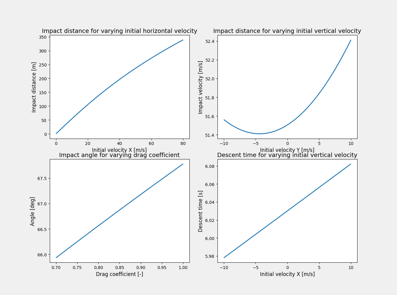
It is possible to do ballistic descent computations with vector input. We do this by setting the initial velocity to an array.
altitude = 150
initial_velocity_x = np.linspace(0, 80, 100)
initial_velocity_y = np.linspace(-10, 10, 100)
However, we cannot have both horizontal and vertical velocities be arrays at the same time, so we use them individually.
p_vel_x = BDM.compute_ballistic_distance(altitude, initial_velocity_x, -2)
p_vel_y = BDM.compute_ballistic_distance(altitude, 30, initial_velocity_y)
The drag coefficient can also be an array.
drag_coef = np.linspace(0.7, 1, 100)
aircraft.set_ballistic_drag_coefficient(drag_coef)
BDM.set_aircraft(aircraft)
p_drag_coef = BDM.compute_ballistic_distance(altitude, 30, -2)
Now p contains the output from each of the three calculations, and this can be plotted to show the variation of the output. Here are some of the possible combination of input and output parameters.
Finally, this example also shows how to get the ballistic computations found in Annex F Appendix A.
This is done by instantiating the AnnexFParms class, since all the ballistic values
are computed internally in the class during instantiation.
AFP = AnnexFParms()
Then we can easily access the associated attributes in the class to get the various ballistic values for each category.
for c in range(5):
    print("{:2d} m      {:3d} m/s     {:4d} m    {:3.0f} m/s   {:3.0f} m/s   {:1.0f} deg    {:4.0f} m     "
          "{:4.1f} s   {:6.0f} kJ".format(
        AFP.CA_parms[c].wingspan, AFP.CA_parms[c].cruise_speed, AFP.CA_parms[c].ballistic_descent_altitude,
        AFP.CA_parms[c].terminal_velocity, AFP.CA_parms[c].ballistic_impact_velocity,
        AFP.CA_parms[c].ballistic_impact_angle, AFP.CA_parms[c].ballistic_distance,
        AFP.CA_parms[c].ballistic_descent_time, AFP.CA_parms[c].ballistic_impact_KE / 1000))
The printed values
Ballistic descent computations
------------------------------
Class   Init horiz     From     Terminal   Impact   Impact   Distance   Descent      KE
          speed      altitude   velocity   speed    angle    traveled    time      impact
 1 m       25 m/s       75 m     25 m/s    24 m/s   76 deg      63 m      4.7 s        1 kJ
 3 m       35 m/s      100 m     45 m/s    39 m/s   64 deg     123 m      4.9 s       39 kJ
 8 m       75 m/s      200 m     63 m/s    60 m/s   57 deg     335 m      6.9 s      718 kJ
20 m      150 m/s      500 m    112 m/s   106 m/s   51 deg    1044 m     10.8 s    27952 kJ
40 m      200 m/s     1000 m    120 m/s   121 m/s   59 deg    1690 m     16.0 s    73038 kJ
are the same as found in the ballistic table in Appendix A of Annex F [1].
- 1
JARUS. JARUS guidelines on SORA - Annex F - Theoretical Basis for Ground Risk Classification. Technical Report, 2022. JAR-WG6-QM.01.
- 2(1,2)
Anders la Cour-Harbo. Ground impact probability distribution for small unmanned aircraft in ballistic descent. In 2020 International Conference on Unmanned Aircraft Systems (ICUAS), 1442–1451. Aalborg University, IEEE, sep 2020. doi:10.1109/ICUAS48674.2020.9213990.