Example 5: Isoparametric critical area plot
This example makes a colored plot of the lethal area for varying impact angles and impact speeds. The size of the aircraft as well as the other parameters are fixed. The idea is to visualize the relation between angle and speed, since this is one of the challenges in understanding the transition from the JARUS model to the iGRC table.
The target for this example is the second column in the iGRC table, where the defined lethal area is 80 m^2. Therefore, the isoparametric curve for 80 m^2 is shown in yellow along with other iso curves in white for comparison.
We start by setting up the critical area class.
CA = CriticalAreaModels()
We instantiate the AnnexFParms class, since we want to use the parameters
for the smallest size aircraft in the iGRC table, and we can find them in that class.
AFP = AnnexFParms()
We then setup the aircraft based on the parmaters for the first column in the iGRC table (thus the index [0] on AFP.CA_Parms). Note that this is not specific for fixed-wing, since this information is not currently being used by the critical area computation.
aircraft_type = enums.AircraftType.FIXED_WING
aircraft = AircraftSpecs(aircraft_type, AFP.CA_parms[1].wingspan, AFP.CA_parms[1].mass)
We do not use any fuel.
aircraft.set_fuel_type(enums.FuelType.LION)
aircraft.set_fuel_quantity(0)
And we use the friction coefficient from Annex F.
aircraft.set_friction_coefficient(AFP.friction_coefficient)
We want to plot over the full range of impact speed and impact angles. However, since very shallow impact angles are not handled well by the model, we start at 5 degrees. For speed, we cap it at 40 m/s. Each axis will be 100 steps, which is fine for a relatively smooth plot.
y_speed = np.linspace(0, 50, 100)
x_angle = np.linspace(5, 70, 100)
X_angle, Y_speed = np.meshgrid(x_angle, y_speed)
We then compute the critical area for all combinations of speed and angle. Note that we could have replaced one of the loops with an array input, but since we cannot replace both (since the critical_area method does not support 2D array input), we have chosen to run both dimensions as loops for code clarity.
Z_CA = np.zeros((X_angle.shape[0], Y_speed.shape[0]))
for i, y in enumerate(Y_speed):
    for j, x in enumerate(X_angle):
        Z_CA[i, j] = CA.critical_area(aircraft, y_speed[i], x_angle[j])[0]
The plot is setup with room for a colorbar on the right.
fig = plt.figure()
ax = plt.axes()
divider = make_axes_locatable(ax)
cax = divider.append_axes('right', size='5%', pad=0.05)
The matrix is added to the plot.
im = ax.imshow(Z_CA, extent=[x_angle[0], x_angle[-1], y_speed[0], y_speed[-1]],
               aspect='auto', origin='lower')
Conturs are added to the plot.
CS = ax.contour(X_angle, Y_speed, Z_CA, [5, 10, 15, 20, 30, 40, 60, 100, 120], colors='white')
ax.clabel(CS, inline=1, fontsize=10, fmt="%u m^2")
A yellow contour is added for the target critical area for the first column in the iGRC table.
CS2 = ax.contour(X_angle, Y_speed, Z_CA, [AFP.CA_parms[1].critical_area_target], colors='yellow')
ax.clabel(CS2, inline=1, fontsize=10, fmt="%1.1f m^2")
And the colorbar is added along with axes labels and title.
fig.colorbar(im, cax=cax, orientation='vertical')
ax.set_xlabel('Angle [deg]')
ax.set_ylabel('Speed  [m/s]')
ax.set_title('Lethal area [m^2] for {:d} m, {:d} kg, {:2.2f} friction'.format(AFP.CA_parms[1].wingspan,
                                                                          AFP.CA_parms[1].mass,
                                                                          AFP.friction_coefficient))
The contours in the output image show where there is a constant critical area for varying combinations of speed and angle.
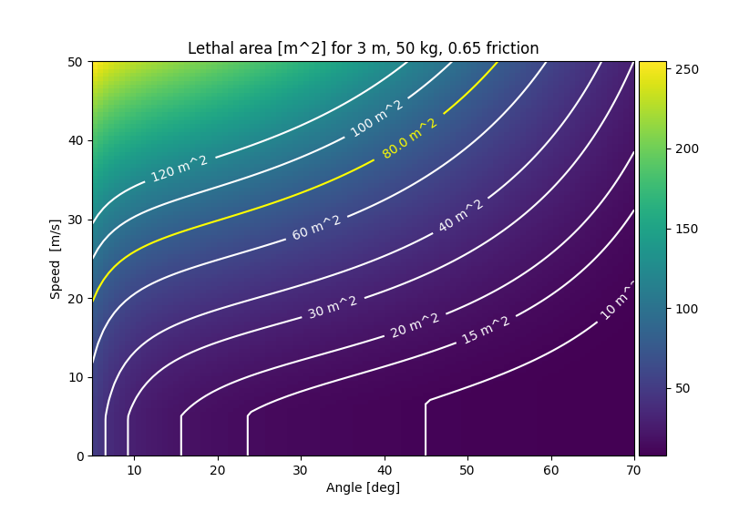
There is a significant “drop” visible for the lower speeds. This is coming from lethal kinetic energy limit described in Annex F, i.e., the disregard of the slide part of the critical area where the slide speed is small enough to have a kinetic energy less than the lethal limit. When the kinetic energy at the start of the slide is less than the lethal kinetic energy, only the glide part is lethal, and this does not depend on speed, only on impact angle. This results in the CA remaining constant for changing speeds for sufficiently low speeds. Consequently, the iso curve becomes vertical in this area.